Immersed Boundary Method

TOSCA implements a sharp-interface, direct-forcing immersed boundary method (IBM) with optional ghost-cells on the inside of the body when wall models are active. The IBM allows complex geometries — terrain features, wind turbine towers and nacelles, and moving objects — to be represented on a structured background grid without mesh deformation. The immersed surface enters the momentum equation through a body-force term \(\mathbf{f}^{IB}\), which is applied implicitly. This means that, at each time step, the velocity (and temperature) field is prescribed at IBM interface cells as a boundary condition rather than an explicit source term in the conservation equations.

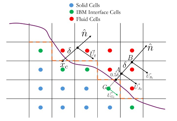
Schematic of the sharp-interface IBM. The immersed surface (triangular mesh, pink line) divides the background grid into fluid cells (red), solid cells (blue), and IBM interface cells (green). Points A and B are the two wall-normal sampling locations used during boundary-condition reconstruction when a wall model is active.

Surface Representation

The immersed-body surface is described as an unstructured triangular mesh provided in STL (.stl) or Abaqus (.inp) format and placed in the IBM/ directory. Multiple bodies can be defined simultaneously in IBM/IBMProperties.dat as object0, object1, etc.

To accelerate cell to element searche, the code builds a two-level spatial data structure during initialisation:

1. Axis-aligned bounding box: a tight box around each body, coarser than the background grid, to accelerate the search.

2. Search-cell list: the bounding box is subdivided into uniform search cells whose size is proportional to the mean element edge length. Every triangular element is inserted into all overlapping search cells. Only elements in the relevant search cells are tested during subsequent point-in-triangle queries, reducing the search cost from \(O(N_e)\) to approximately \(O(1)\).

Cell Classification (Topology Check)

Every background-grid cell is classified into one of three categories by a ray-casting algorithm. In particular, a ray is cast from each cell centre and the number of intersections with the triangular IBM surface is counted.

• Fluid cell: even number of intersections, the cell lies outside the body.

• Solid cell: odd number of intersections, the cell lies inside the body.

• IBM interface cell: any solid cell immediately adjacent to at least one fluid cell. These cells are not advanced by the flow solver. Instead, their field values are overwritten each time step by the IBM boundary-condition reconstruction.

For each IBM interface cell, the code identifies the closest triangular element and stores its outward unit normal \(\hat{\mathbf{n}}\) and the projection of the cell centre onto the surface, the so-called wall point \(\mathbf{p}_\text{w}\). The closest-element search uses a bounding-sphere acceleration: each element’s circumsphere centre \(\mathbf{q}\) and radius \(r\) are pre-computed, and the element with the smallest value of \(\|\mathbf{x} - \mathbf{q}\| - r\) is selected as the closest candidate before the precise face/edge/vertex projection is performed.

Boundary-Condition Reconstruction

Two reconstruction modes are available, selected via wallShearOn and the corresponding velocityBC in the IBMProperties.dat file.

Without Wall Model

When wallShearOn is set to false and velocityBC is slip or noSlip, the IBM interface cell velocity is set by one-point interpolation. A single background point B is placed at a distance \(\delta\) along \(\hat{\mathbf{n}}\) from the centre of the IBM interface cell. The parameter \(\delta\) equals the minimum local cell size (for the CurvibTrilinear interpolation) or the distance to an interception point on an adjacent grid plane (for the CurvibTriangular interpolation). Denoting the wall-normal distances from the IBM surface as \(s_{ic}\) (IBM interface cell) and \(s_b\) (background point B), the velocity reconstruction at the IBM interface cell gives

\[\mathbf{u}^{ic} = \frac{s_{ic}}{s_b}\,\mathbf{u}_B + \left(1 - \frac{s_{ic}}{s_b}\right)\mathbf{u}_\text{wall},\]

where \(\mathbf{u}_\text{wall}\) is the IBM-surface velocity interpolated from the triangular mesh nodes using barycentric weights. For a slip boundary, the normal component at the IBM interface cell is scaled with the ratio \(s_{ic}/s_b\) in order to enforce no penetration, while the tangential component is left unchanged. The IBM surface velocity is then added to the reconstructed velocity to account for any motion of the body.

With Wall Model

When wallShearOn = true and velocityBC = velocityWallFunction, the reconstruction uses two background sampling points placed at distances \(s_c\) and \(s_d\) from the IBM wall, and a ghost node placed at \(s_g\) Setting \(\delta = \texttt{interpDist}\):

\[s_g = -0.5\delta, \qquad s_a = 0.5\delta, \qquad s_b = 1.5\delta,\]

The arrangement along the wall normal is therefore

\[G \;\cdots\; \text{wall} \;\cdots\; A \;\cdots\; B.\]

Velocities at B (\(\mathbf{u}_B\)) is obtained by trilinear interpolation from the background grid, while the velocity at A is given by

\[\mathbf{u}_A = \mathbf{u}_B\frac{ln\left(0.5\delta/z_0\right)}{ln\left(1.5\delta/z_0\right)},\]

where \(z_0\) denotes the surface roughness length. The ghost-cell velocity at point G is then linearly extrapolated from point A and B, correcting the wall-normal component to enforce no penetration at the IBM surface.

In addition to the velocity reconstruction, a modeled wall shear stress is also reconstructed at faces shared by an immersed-body interface cell and a neighboring fluid cell. Let \(\boldsymbol{\mathsf{n}}\) denote the unit normal to the closest immersed-body surface triangular element associated with the IBM interface cell, and let \(\boldsymbol{\mathsf{u}}\) denote the fluid velocity sampled at a distance \(\delta\) from the surface along \(\boldsymbol{\mathsf{n}}\). For isotropic grids, \(\delta=\Delta\), where \(\Delta\) is the grid spacing, whereas for anisotropic grids, \(\delta\) represents the approximate local grid spacing in the wall-normal direction.

The tangential component of the sampled velocity is obtained using the projection operator

\[\mathbb{P}_t = \mathbb{I} - \boldsymbol{\mathsf{n}} \otimes \boldsymbol{\mathsf{n}}, \qquad \boldsymbol{\mathsf{u}}_t = \mathbb{P}_t\,\boldsymbol{\mathsf{u}}, \qquad u_t = \lVert \boldsymbol{\mathsf{u}}_t \rVert .\]

Then, a local orthonormal coordinate frame aligned with the immersed-body surface is defined as

\[\boldsymbol{\varepsilon}_1 = \frac{\boldsymbol{\mathsf{u}}_t}{u_t}, \qquad \boldsymbol{\varepsilon}_2 = \boldsymbol{\mathsf{n}} \times \boldsymbol{\varepsilon}_1, \qquad \boldsymbol{\varepsilon}_3 = \boldsymbol{\mathsf{n}},\]

with corresponding rotation matrix

\[\mathbf{Q} = \big[\,\boldsymbol{\varepsilon}_1\;\boldsymbol{\varepsilon}_2\;\boldsymbol{\varepsilon}_3\,\big],\]

which maps quantities between the global and local wall-parallel coordinate systems.

Assuming that the tangential velocity follows a rough-wall logarithmic profile, the magnitude of the wall shear stress is given by

\[\tau_w = \left[ \frac{\kappa\,u_t}{\ln\!\left(\delta/z_0\right)} \right]^2,\]

where \(\kappa = 0.4\) is the von Karman constant. Although the face center \(x_c\) does not, in general, lie on the immersed-body surface, the quantity \(\tau_w\) is taken to represent the \(\mathcal{T}_{13} = \mathcal{T}_{31}\) component of the shear stress tensor in the local coordinate system, with all other components set to zero. Accordingly, the local shear stress tensor \(\mathcal{T}^{(\mathrm{loc})}\) is expressed as

\[\mathcal{T}^{(\mathrm{loc})} = \tau_w \big( \boldsymbol{\varepsilon}_1 \otimes \boldsymbol{\varepsilon}_3 + \boldsymbol{\varepsilon}_3 \otimes \boldsymbol{\varepsilon}_1 \big).\]

The corresponding stress tensor imposed at the immersed-body interface face in the global coordinate system is obtained through the transformation

\[\mathcal{T} = \mathbf{Q}\, \mathcal{T}^{(\mathrm{loc})}\, \mathbf{Q}^{\!\top}.\]

This stress is applied only at immersed-boundary interface faces and is set to zero inside the immersed- body.

Wall Models

The wall boundary condition for velocity and temperature is configured per-body in IBMProperties.dat, or matched from a domain boundary face via velocityBCSetType = matchU*.

Velocity Wall Models

Type	Name	Description
-1	Cabot	Neutral log-law with optional aerodynamic roughness kRough. The friction velocity \(u_*\) is solved iteratively from \(u_t = (u_*/\kappa)\ln[(1.5\delta + z_0)/z_0]\). The smooth-wall limit is recovered when kRough = 0.
-3	Schumann	Stability-corrected log-law. The relation \(u_t = (u_*/\kappa)[\ln(1.5\delta/z_0) - \psi_m(1.5\delta/L)]\) is used, where \(L\) is the Obukhov length and \(\psi_m\) is the Monin–Obukhov stability function. Must be paired with the Schumann temperature wall model (-2 or -4) when temperature is active.
-4	Power-law APG	Power-law wall profile for adverse-pressure-gradient flows.
-5	Log-law APG	Log-law wall profile for adverse-pressure-gradient flows.

Temperature Wall Models

Type	Name	Description
-2	Shumann — constant flux	Prescribed constant wall heat flux qWall \([\mathrm{K\,m\,s^{-1}}]\).
-3	Shumann — heating rate	Prescribed constant surface heating rate (Not yet implemented for IBM).
-4	Shumann — time history	Surface potential temperature and Obukhov length read from a time-series file (readSurfaceTempData). The IBM interface cell temperature is interpolated linearly between the IBM surface temperature (looked up at the current time) and the value at point A.

In addition to thetaWallFunction, the temperature boundary condition at an IBM surface can be set to zeroGradient (IBM interface cell temperature equals the value at A) or fixedValue (IBM interface cell temperature equals the prescribed as fixedValueT).

Interpolation Schemes

The interpolation model is selected via IBInterpolationModel in IBMProperties.dat. The available options and their governing functions are listed below.

IBInterpolationModel	curvibType	curvibOrder	Function / Notes
CURVIB	CurvibTrilinear	linear	CurvibInterpolation — one background point at one minimum cell size along \(\hat{\mathbf{n}}\). Supports Cabot, Schumann, slip, noSlip boundary conditions.
CURVIB	CurvibTrilinear	quadratic	CurvibInterpolationQuadratic — as above but uses a quadratic wall-normal profile.
CURVIB	CurvibTriangular	—	CurvibInterpolationTriangular — the image point is the intersection of the wall-normal ray with an adjacent curvilinear grid plane, barycentric weights of the enclosing triangle are used for interpolation. Supports the same boundary conditions as trilinear.
CURVIB + wallShearOn	—	—	CurvibInterpolationInternalCell — two background points, full hybrid wall-shear reconstruction with quadratic pressure extrapolation.
MLS	—	—	MLSInterpolation — Moving Least Squares reconstruction over a cloud of fluid support nodes identified by findFluidSupportNodes and findIBMMeshSupportNodes.

Note

The wallShearOn flag requires IBInterpolationModel = CURVIB and a velocityBC = velocityWallFunction entry. It overrides the curvibType / curvibOrder settings and always uses CurvibInterpolationInternalCell.

Dynamic IBM

Setting dynamic = true in IBMProperties.dat enables a moving immersed body. At every time step UpdateIBM rebuilds the full cell-classification data structures:

1. Previous lists are destroyed (destroyLists).

2. The mesh is advanced by UpdateIBMesh (see motion types below).

3. The bounding box, search-cell list, outward normals, ray-casting classification, IBM fluid-cell list, and closest-element search are all recomputed from scratch.

This per-step re-initialisation supports arbitrarily large motions with no restriction on the displacement per time step. Operations are parallelised with MPI so that, after the initial search, IBM searches at subsequent steps are only performed in the vicinity of the previous body position.

The mesh motion is performed by UpdateIBMesh, which dispatches to the following bodyMotion types:

bodyMotion	Description
static	No motion; lists are built once at initialisation and not rebuilt.
rotation	Rigid rotation about rotCenter and rotAxis at angular speed angSpeed \([\mathrm{rad\,s^{-1}}]\). The speed may ramp at a constant rate angAcc \([\mathrm{rad\,s^{-2}}]\). Node coordinates and velocities are updated by rotateIBMesh. The instantaneous angular position is written to fields/<mesh>/ibm/<time>/<bodyName>.
sinusoidal	Sinusoidal translation along motionDir with amplitude \(A\,[\mathrm{m}]\) and frequency \(f\,[\mathrm{Hz}]\). The displacement applied each step is \(A\bigl(\cos 2\pi f t_\text{prev} - \cos 2\pi f t\bigr)\).
pitchingOscillation	Sinusoidal pitching rotation about pitchCenter / pitchAxis with amplitude \(A\,[\mathrm{rad}]\) and frequency \(f\).

Force and Moment Integration

When computeForce = true, the aerodynamic load on each IBM object is evaluated every timeInterval (or physical-time interval, depending on intervalType) by ComputeForceMoment. For each triangular element of the IBM surface mesh the procedure is:

1. A pressure-interpolation point is placed at a distance \(\ell = \sqrt{2\,A_e}\) (where \(A_e\) is the element area) outward from the element centre along \(\hat{\mathbf{n}}\). If that point lies inside solid cells it is shifted outward in increments of \(0.2\,\ell\) until a valid trilinear interpolation stencil is found.

2. The static pressure \(p\) and velocity \(\mathbf{u}\) are trilinearly interpolated at the interpolation point.

3. The pressure force on the element is calculated as

   \[\mathbf{F}_P^{(e)} = -\rho\!\left(p - \frac{\partial u_{\text{wall},n}} {\partial t}\,\ell\right)A_e\,\hat{\mathbf{n}},\]

   where \(u_{\text{wall},n} = \partial\mathbf{u}_\text{wall}/\partial t \cdot\hat{\mathbf{n}}\) is the IBM-surface normal acceleration, which provides a correction for the unsteady pressure gradient next to a moving wall.

4. The viscous shear force is computed from the friction velocity \(u_* = u_\tau(\mathbf{u}_B - \mathbf{u}_\text{wall})\) using the Cabot model and applied in the direction of the relative tangential velocity.

Net pressure force, viscous force, aerodynamic torque, and shaft power (for rotation bodies) are reduced across all MPI ranks and appended to

postProcessing/<meshName>/IBM/<startTime>/<bodyName>/netForce/<bodyName>_netForce

Per-element pressure loads (in Abaqus .dlo format) are written to the elementForce/ subfolder when writePForce = true in the io sub-dict.