Neutral ABL Example

The tests/NeutralABLTest example case shows how to simulate a conventionally neutral atmospheric boundary layer (CNBL) in TOSCA. CNBLs are characterized by a strong capping inversion layer of thickness \(\Delta h\), across which a potential temperature jump \(\Delta \theta\) is observed. Stratification is neutral below the inversion layer, while it is characterized by a linear lapse rate \(\gamma\) aloft.

These types of flows are simulated using lateral periodic boundary conditions, while the flow driven by a large-scale driving pressure gradient imposed using TOSCA’s velocity controller. In this example, the pressure controller is used, which controls the large-scale horizontal pressure gradient in order to obtain a wind speed of 8 m/s at the height of 90 m.

The flow is initialized using a logarithmic profile below the inversion height \(H\), and a uniform wind above. As the simulation progressess, turbulence is created and starts developing inside the flow domain. To accelerate this process, spanwise fluctuations can be imposed in the initial flow to anticipate turbulence onset.

All the above aspects can be controlled from the ABLProperties.dat file (see Sec. ABLProperties.dat for a detailed description of all entries). In particular, entries controlling the initial temperature and velocity profile are defined by the following parameters:

uRef    8.0    # wind speed at hRef in m/s
hRef    90.0   # reference height in m
tRef    300.0  # ground potential temperature in K
hRough  0.003  # equivalent roughness length in m
hInv    750.0  # height of the inversion center in m
dInv    100.0  # width of the inversion center in m
gInv    5.0    # potential temperature jump in K across inversion
gTop    0.003  # gradient of the linear lapse rate above inversion in K/m
gABL    0.0    # gradient of the linear lapse rate below inversion in K/m (zero for neutral)
vkConst 0.4    # value of the Von Karman constant
smearT  0.33   # defines the smearing of the initial potential temperature profile

Then, the following flags are set in order to activate the velocity controller, the temperature controller (which maintains constant the horizontally averaged potential temperature profile, preventing the inversion layer to displace upwards), the Coriolis force and the initial flow perturbations in the velocity field:

controllerActive  1               # activates velocity controller
controllerActiveT 1               # activates temperature controller
controllerTypeT   initial         # target temperature is the initial temperature
coriolisActive    1               # activates Coriolis force
fCoriolis         5.156303966e-5  # 2 times the Coriolis parameter
perturbations     1               # flow perturbations

Notably, the fCoriolis should be set to \(7.272205217\cdot 10^{-5} \sin(\phi)\) (2 times the Coriolis parameter), where \(\phi\) is the latitude. This is a TOSCA convention and other codes do the multiplication by 2 internally. Finally, the parameters defining the velocity controller must be specified in the controllerProperties dictionary, namely

controllerProperties
{
    controllerAction     write    # controller writes the momentumSource inside
                                  # postProcessing/
    controllerType       pressure # controller tries to maintain uRef at hRef
    relaxPI              0.7      # proportional gain
    alphaPI              0.9      # proportional over integral ratio
    timeWindowPI         3600     # time constant of the controller low-pass filter
    geostrophicDamping   1        # only for pressure controller, eliminates inertial
                                  # oscillations
    geoDampingAlpha      1.0      # alpha 1 corresponds to critical damping
    geoDampingStartTime  5000     # should start damping after turbulence has developed
    geoDampingTimeWindow 4500     # should be large (ideally one inertial oscillation)
    controllerMaxHeight  100000.0 # the controller is applied in the entire domain
}

In order to tell TOSCA to initialize the flow using the parameters defined within the ABLProperties.dat file, the internalField keyword inside the boundary condition files boundary/U, boundary/T and boundary/nut should be set to ABLFlow. More details regarding the optimal setup for these types of simulations in the context of larger cases can be found here .

Checking the case

In order to check that everything is correct, we run TOSCA for just one second and check the resulting fields in ParaView. In order to do so, the following entries should be edited in the control.dat file

-startFrom                 startTime
-startTime                 0
-endTime                   1
-adjustTimeStep            0
-timeStep                  0.5

-timeInterval              1

-sections                  0

This will stop the simulation after 2 iterations of 0.5 s each (i.e. 1 s of simulation). Notably, the flow sections are also deactivated, as two seconds of simulation will not produce any with the specific settings defined in the sampling directory of this example case. Once TOSCA executables tosca and tosca2PV are copied inside the case directory, TOSCA can be run in serial using

./tosca

or in parallel (using 4 processors) with

mpirun -np 4 ./tosca

Once the initial test completes, the user should first check that the entry -postProcessFields is active in the control.dat file, then run

./tosca2PV

The last executable creates an new XMF directory in which the solution fields are stored in .hdf format. The log file gives information about what fields are written, and should look as follows:

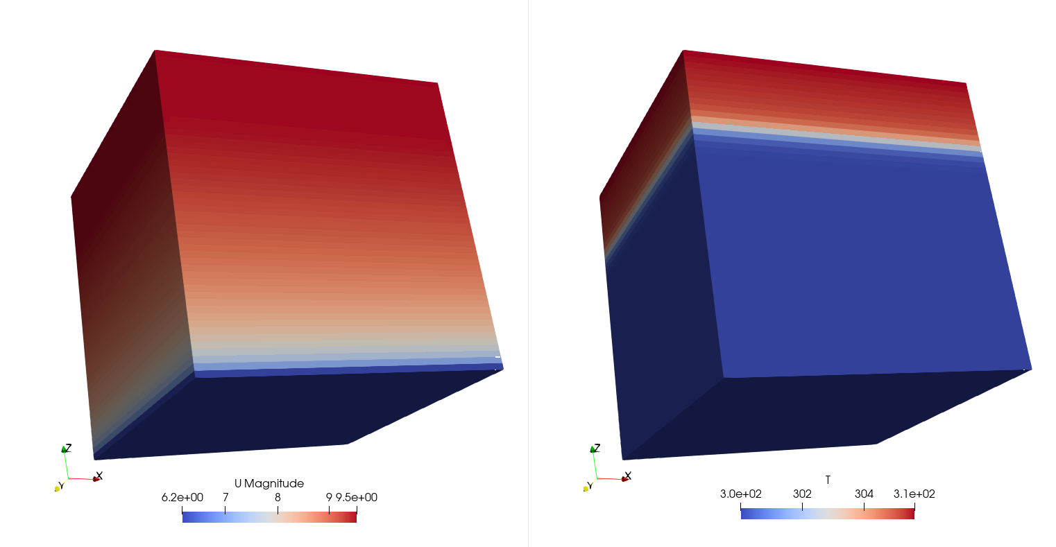
In order to visualize the data, the user should navigate inside the XMF directory and open the .xmf file e.g. using ParaView. The following image shows the result of this operation. In particular, velocity and potential temperature fields are depicted on the left and right panels, respectively.

Turbulence spinup phase

Now the actual simulation can be started. In particular, the turbilence spinup phase should be first carried out. This is required to reach statistical independence of the turbulent fluctuations and, although it does not produce any meaningful data, it is required before one can start to gather flow statistics and sampling sections. To this end, the following parameters should be edited in the control.dat file:

-startFrom                 startTime
-startTime                 0
-endTime                   10000
-adjustTimeStep            1

-timeInterval              500

-sections                  0
-probes                    0
-averageABL                1
-average3LM                0
-avgABLPeriod              10
-avgABLStartTime           0

-averaging                 0
-avgPeriod                 50
-avgStartTime              1000

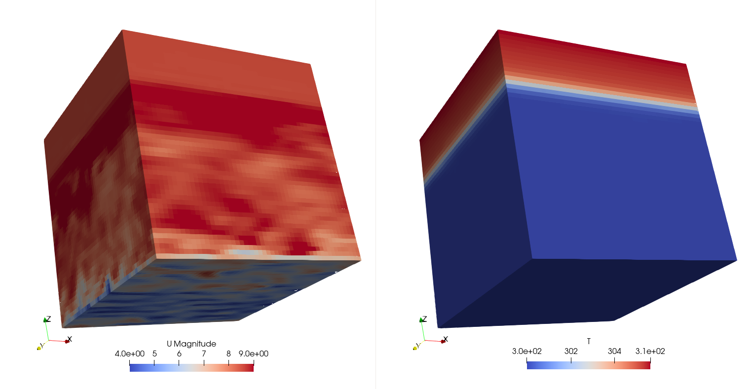
After launching tosca, the simulation will restart from time 0, and run for 10000 s. The time step will be adjusted based on the CFL value and in order to average ABL fields every 10 s. The user can notice that every 500 s a new time directory is created inside the fields directory. Here, checkpoint files are saved for post processing or simulation restart. Moreover, ABL averages (planar averages of different flow quantities at every height) are stored every 10 s inside the postProcessing/averaging/<startTime> directory. The figure below shows the velocity (left) and temperature fields (right) at the end of the spinup phase.

Data acquisition phase

At this point, the simulation can be restarted from 10000 s and flow statistics can be gathered. Usually, precursor simulations are used to save flow sections of velocity, temperature and effective viscosity at each time step, which are then assembled into an inflow database and later used as inlet boundary condition for a subsequent simulation, e.g. with wind turbines. If this is the case, or if the user simply desires to visualize flow planes, sampling planes should be activated in the control.dat file by setting the -sections flag to 1. Saving sections is also useful for large cases, when the domain is too large to be visualized in its entirety as it does not fit in the available RAM memory of a laptop (or even a single supercomputer node).

When sampling planes are later used as inlet boundary conditions, this will happen in TOSCA at the kLeft boundary, as it is the only boundary that features special inlet functions (see Sec. Inlet Functions for details). Hence, the settings of kSections have to be such that these are written with the highest possible frequency to reduce the error of their interpolation in time when used as inflow. Hence, the sampling/surfaces/kSections file is usually defined with the following syntax:

surfaceNumber 1         # one k-surface
timeStart     10000     # acquisition starts at 10000
intervalType  timeStep  # writes every timeInterval iterations
timeInterval  1         # writes every iteration
coordinates   10.0      # plane located at x = 10 m

Conversely, sections used for visualization (usually iSections and jSections, but also kSections can be visualized) are sampled less frequently. For example, a possible syntax for the sampling/surfaces/jSections file is given below.

surfaceNumber 2               # two j-surface
timeStart     1000            # acquisition starts at 10000
intervalType  adjustableTime  # writes every timeInterval seconds
timeInterval  10              # writes every 10 seconds
coordinates   90.0  500.0     # flow section at hub and inversion heights

In is important now to tell TOSCA to read the saved checkpoint file at the latest time, otherwise it will re-initialize the flow using the input parameters defined in ABLProperties.dat. To this end, and in order to terminate the simulation at 12000 s, the control.dat can be edited as follows:

-startFrom    latestTime      # reads the latest time inside the fields directory
-endTime      12000           # simulate 2000 more s with data acquisition

In addition, the internalField entry in the boundary files has to be changed to readField (in all U, p and nut files). The simulation is now set up for restart, and subsequent restarts will not require further editing until the final time is reached. Finally, 3D field averaging and the sampling sections are activated by setting

-sections                  1
-averageABL                1
-avgABLPeriod              10
-avgABLStartTime           0

-averaging                 1
-avgPeriod                 5
-avgStartTime              10000

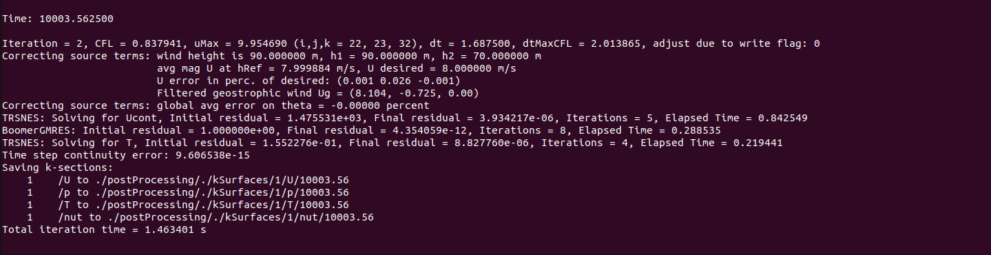
in the control.dat file. Once TOSCA is submitted, the user can verify from the log file (see below) that kSections are stored every iteration inside the postProcessing/kSurfaces/k-ID directory, where k-ID corresponds to the k-index of the plane of cells intercepts by the sampling surface . Notably, the name of each section file corresponds to the time at which the section has been taken, where the number of decimal places can be controlled with the -timePrecision keyword in the control.dat file.

Once that the simulation completes, all data except from the 3D fields are stored inside the postProcessing directory. In particular, iSections, jSections, kSections and ABL averages at different levels are stored in the here, while 3D field averages and checkpoint variables are located in the corresponding checkpoint time inside the fields directory. As this test case is small, the user can decide to visualize them in e.g. ParaView by running tosca2PV. For large simulations, these files are usually kept for hypotetically restarting the simulation at a later phase, if needed. However, 3D field averages can be sliced after the simulation using TOSCA’s post processor tosca2PV. This is done by leaving both the -averaging and the -sections flags activated control.dat file, prompting the code to re-read the definition of the sampling sections and then slice the average fields.

Currently, no additional sections can be added a-posteriori if instantaneous sections (generated during the simulations) are found inside the postProcessing directory. In order force tosca2PV to re-read the section definitions inside sampling (i.e. after adding more sections) and re-slice the 3D average fields, it is sufficient to rename the directories postProcessing/iSurfaces, postProcessing/jSurfaces or postProcessing/kSurfaces to something else, depending if sampling/surfaces/iSections, sampling/surfaces/jSections or sampling/surfaces/kSections have been edited, respectively. This procedure is identified in TOSCA as on-the-fly section re-acquisition, and it is printed in the terminal (or the log file) when running tosca2PV.

Regarding the data contained in the postProcessing directory - except from sections, which are read using tosca2PV - this is usually post processed using ad-hoc Python or Matlab scripts.

Creating the inflow database

In order to create an inflow database that can be later used by TOSCA, the workflow is the following.

1. Create a directory named inflowDatabase.

2. Copy the directories U, T (if present) and nut, contained inside the directory postProcessing/kSurfaces/k-ID/, where the k-ID corresponds to the kSurface selected for sampling the inflow data, inside the inflowDatabase directory.

3. Create a new file named momentumSource inside the inflowDatabase directory. Then copy the content of each postProcessing/momentumSource_<startTime> file inside the momentumSource file, eliminating the overlapping portion of each source file’s time history (as if source files were tiled together).

4. Copy the mesh.xyz file inside the inflowDatabase directory, renaming it inflowMesh.xyz. In this file, eliminate the lines -iPeriodicType, -jPeriodicType and -kPeriodicType, if present.

The inflowDatabase is now a standalone inflow database that can be used as inlet boundary condition for several different successor simulations.