NREL 5MW Example - Uniform Flow
In the tests/NREL5MWTest example case, the NREL 5MW wind turbine is simulated using the ADM, with a uniform inflow of 20 m/s. To make the example case more interesting, the wind turbine is initially placed such that the rotor plane is parallel to the wind direction, and the yaw controller slowly rotates the turbine such that it faces the wind direction. As the rotor gradually takes up more wind, the pitch controller adjusts the pitch angle to protect the wind turbine above rated conditions.
This example shows the usage of user-defined sections (see Sec. -sections), field averaging (see Sec. -averaging and -phaseAveraging) and the acquisition of mechanical energy budgets (see Sec. -keBudgets).
The simulation is run for 500 s with adaptive time stepping and checkpoint files written every 100 s. These parameters are set in the
control.dat file as follows:
-startFrom      startTime
-startTime      0
-endTime        500
-cfl            0.8
-adjustTimeStep 1              // adjust time step based on CFL and write frequency
-timeStep       0.5            // initial time step

-intervalType   adjustableTime // time step adjusted based on write frequency
-timeInterval   100            // write frequency
The domain extends from -250 to 250 m in the x and y directions, while it goes from -90 to 210 m in the z. The wind turbine, which has a hub-height
of 90 m, is such that the rotor center is located at (0, 0, 0), as defined in the turbines/windFarmProperties file. The rotor is represented using
the ADM, and turbine data are written to file at every iteration. In order initially misalign the wind turbine by 90 degrees, the user should modify
the direction of the rotor plane in the turbines/NREL5MW file as follows:
rotorDir (0.0 1.0 0.0)
and note that all turbine controls are activated. The initial state of the wind turbine (rotation and pitch) corresponds to the turbine state when
the wind is stationary at 9 m/s, so the controller will try to adjust to the new condition. Moreover, the initial misalignment angle should be
changed to 90 degrees inside the yawControllerParameters in the turbines/control/fiveRegionsNREL file as follows:
initialFlowAngle 90
Finally, the inflow wind speed should be changed from 5 m/s (as per the original test case) to 20 m/s. This is done by editing the kLeft
boundary condition in the boundary/U fileas follows:
kLeft fixedValue (20.0 0.0 0.0)
Sections, averages and mechanical energy budgets are activated in the control.dat file as follows:
-sections        1      // TOSCA reads inside sampling/surfaces

-averaging       1      // write avgCs, avgNut, avgP, avgU and avgUU at checkpoints
-avgPeriod       0.5    // cumulate averages every 0.5 s
-avgStartTime    100    // start averaging after 100 s

-keBudgets       1      // TOSCA reads sampling/keBudgets file
The sampling/surfaces directory contains the userSections directory, where three arbitrary sections are defined, as well as
curvilinear sections defined inside iSections and jSections files. As the mesh is cartesian, these correspond to y-normal and
z-normal slices, respectively. Only one section is defined per file in this case, both cutting the rotor plane at the hub height.
The sampling/keBudgets file, only activated to show its usage (it has no real meaning, similarly to the field averaging, as the
simulation is unsteady), contains three boxes of size 80x80x80 m, centered at the rotor center, 80 m and 160 m downstream. These can
be defined as follows:
avgStartTime  0
avgPeriod     2
debug         0
cartesian     1

boxArray
{
    B1
    (
        boxCenter (0.0 0.0 0.0)
        sizeXYZ   (80.0 80.0 80.0)
    )
    B2
    (
        boxCenter (80.0 0.0 0.0)
        sizeXYZ   (80.0 80.0 80.0)
    )
    B3
    (
        boxCenter (160.0 0.0 0.0)
        sizeXYZ   (80.0 80.0 80.0)
    )
}
At this point, after copying the tosca and tosca2PV executables inside the case directory, the simulation can be started using 4 processors:
mpirun -np 4 ./tosca
While the simulation runs, the user can open the postProcessing/turbines/A1 file to monitor the behavior of the wind turbine. As can be noticed,
the yaw controller slowly rotates the turbine such that it faces the wind direction, while the commanded pich gradually increases.
After the simulation has completed, the results can be visualized using the tosca2PV executable:
./tosca2PV
Notably, the average fields are now written for both the curvilinear and user-defined sections, as testified by the tosca2PV output.
The following plot, created from the content of the postProcessing/turbines/0.00/A1 file, shows the adjustment of the wind turbine variables
to the initial 90 degs misalignment.
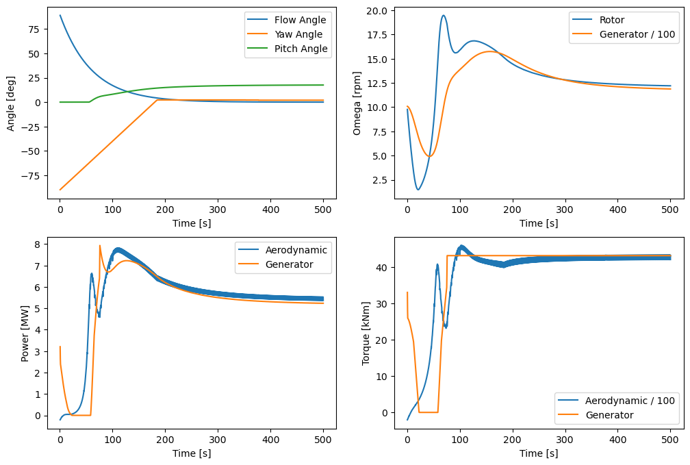
Interstingly, the controller switches off the wind turbine for a few seconds, during the transition phase. As designed, the controller drives the wind turbine to face the wind direction, while the pitch controller adjusts the pitch angle to protect the wind turbine above rated conditions, while the power output adjusts to 5 MW.
After running the tosca2PV executable, the user can visualize the results using ParaView. In particular, the executables creates the XMF directory,
which contains the NREL5MW.xmf file (where all saved 3D fields from all checkpoints are contained) as well as the iSections, jSections and
userSections directories. The first two will contain, in addition to the sliced average fields, also the instantaneous sections saved during the
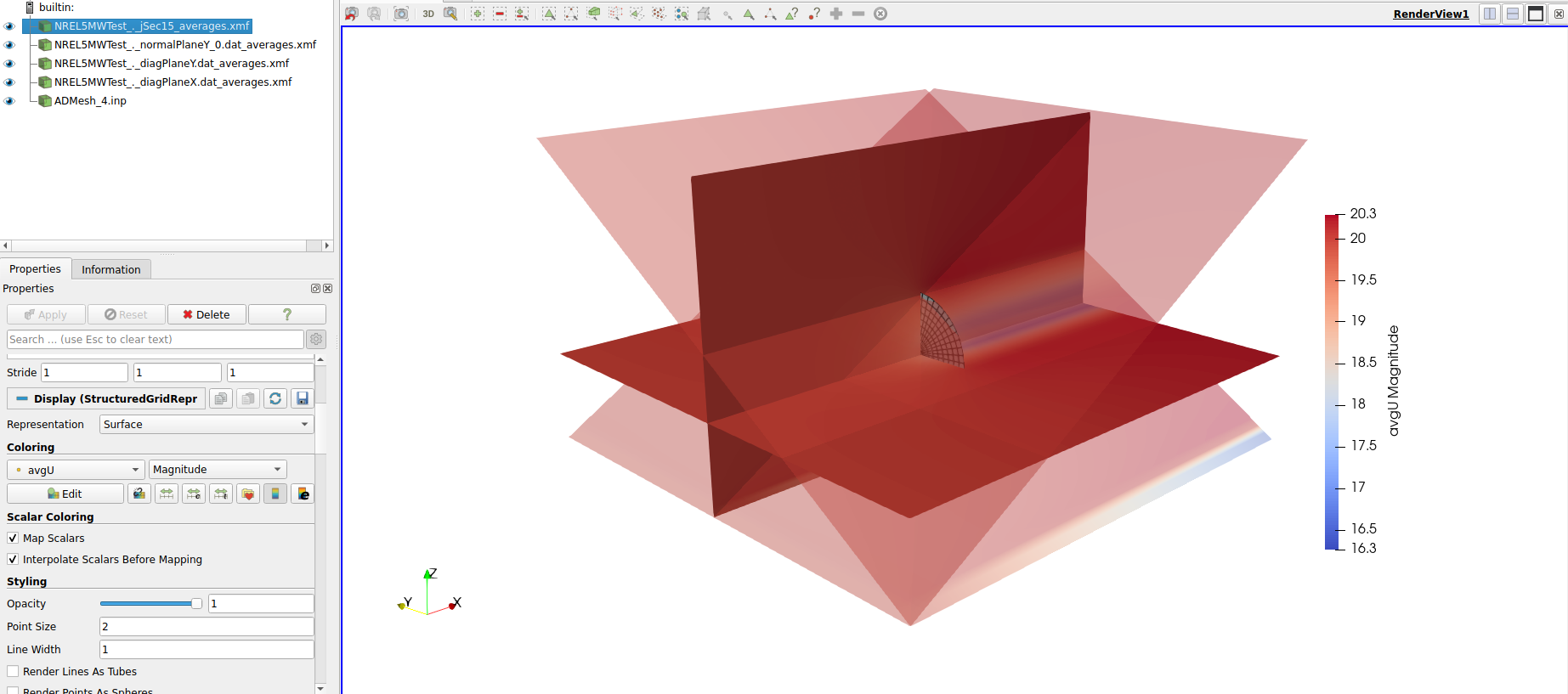
simulation. Conversely, userSections will only contain the average fields for the user-defined sections (three in this case). The following image shows
the average velocity magnitude on all sections defined in the simulation, as well as the final position of the rotor disk. This is written at every
checkpoint file inside the postProcessing/turbines/0.00 directory.
By loading the instantaneous z-normal sections inside the postProcessing/jSections/0.00 directory into ParaView, the
user can create the following video, which shows the evolution of the instantaneous velocity and pressure fields over time.
Finally, the mechanical energy budgets are written inside the postProcessing/keBoxes/0.00 directory, where file for each box is created. This utility,
just shown here for demonstration purposes, can be used to track the mechanical energy budgets of the flow moving through e.g. a wind farm, by suitably
defining the boxes and plotting the various contributions to the mechanical energy equation box by box.